Blog

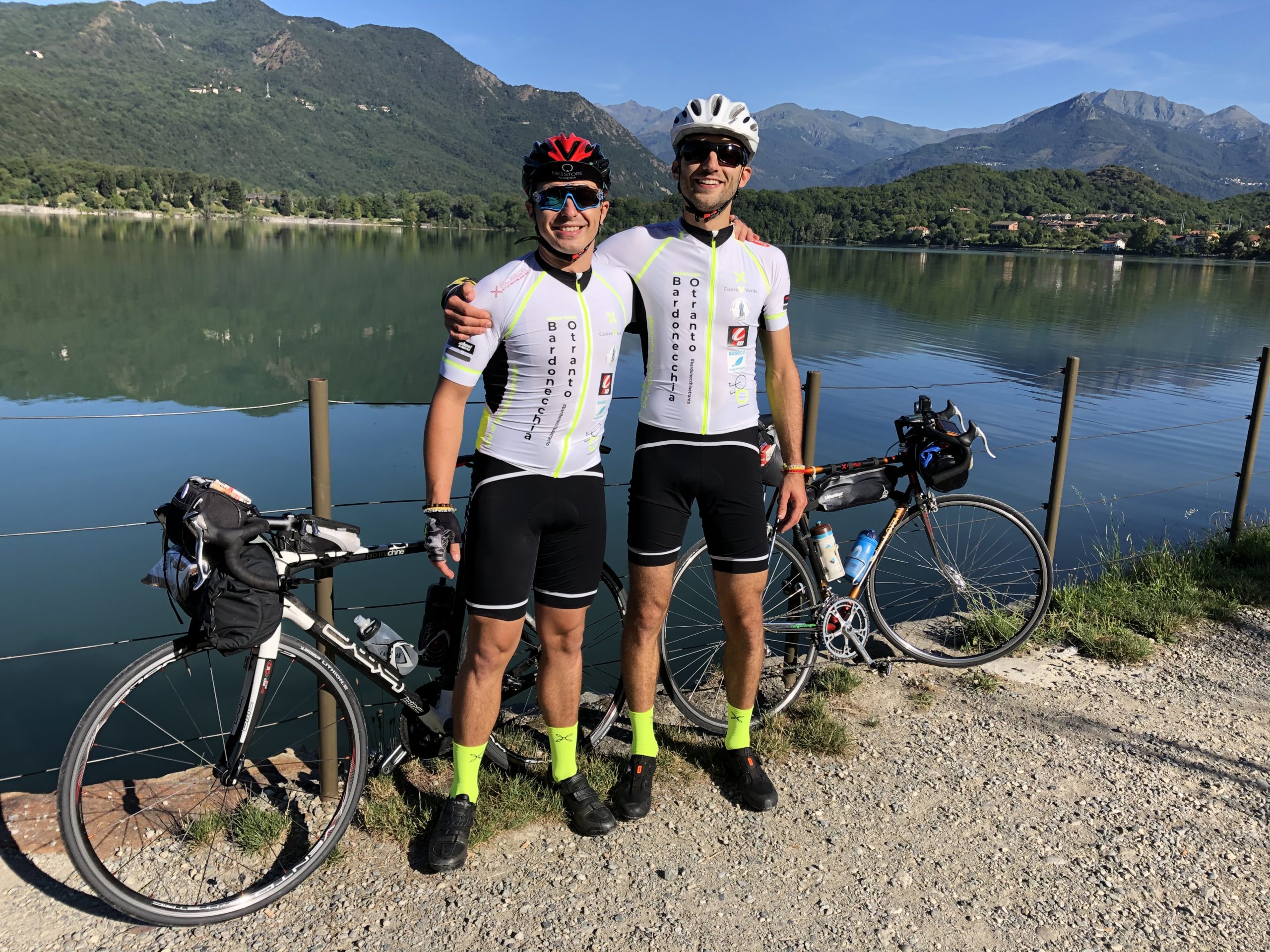
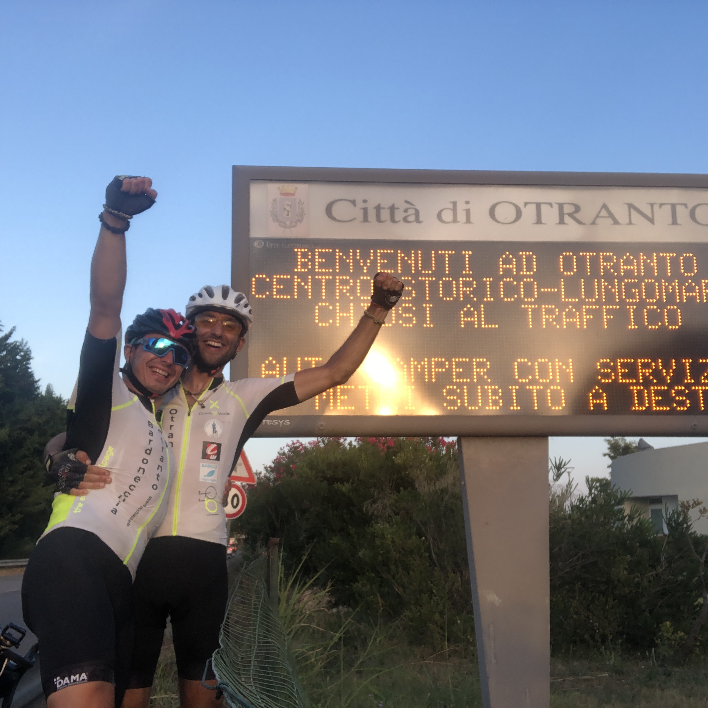
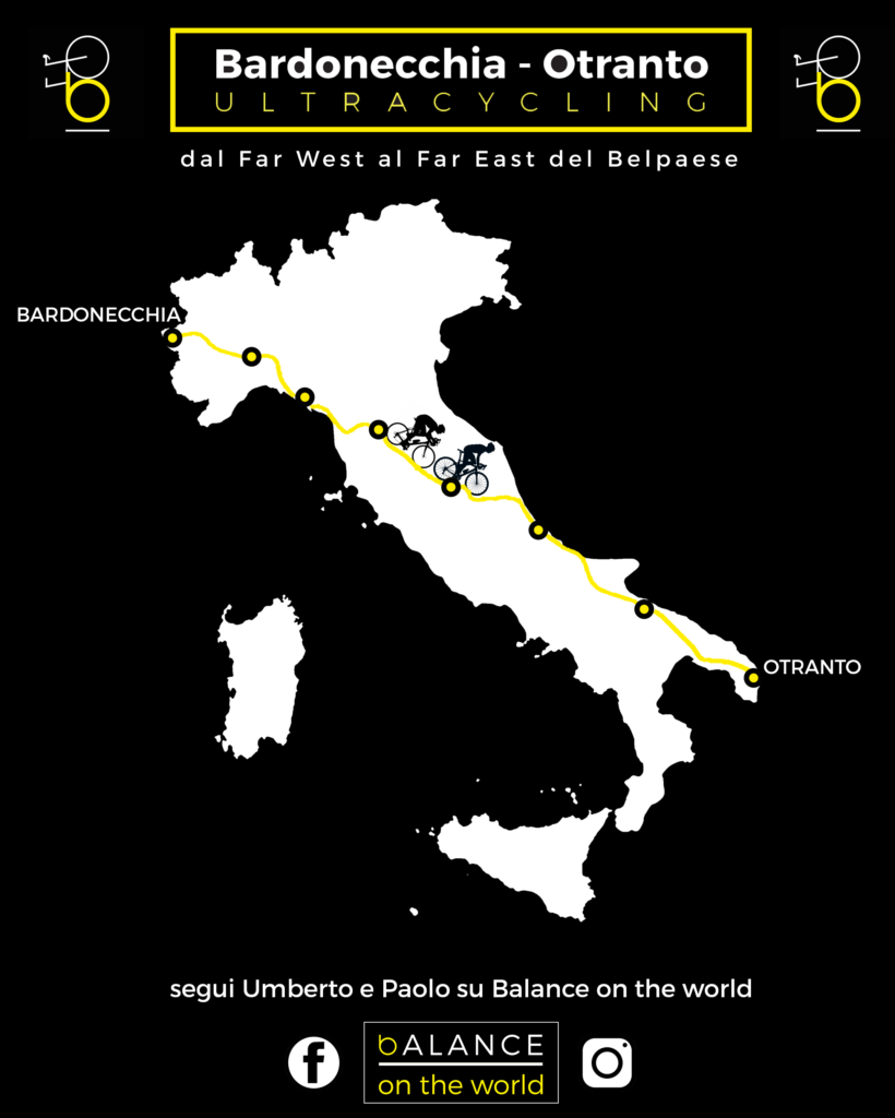
After reading about Umberto’s amazing cycling experience across Italy in the last blog entry, we sadly had to admit that summer was really over. Then it is really time to sit again at your school desk and deal with a more technical topic. Therefore, this time I would like to introduce you to the basics of the Extended Finite Element Method or X-FEM. What does the extension in X-FEM stand for? Or, if you rather, what is the X factor of X-FEM?

Originally proposed by A. Hansbo and P. Hansbo [1], X-FEM is an advanced numerical technique that extends the range of applications of the more classical Finite Element Method (FEM), thanks to its geometric flexibility and the preservation of its accuracy even in complex topological configurations.
Before explaining the reasons for this gain in X-FEM, I first need to recall the main concepts in FEM theory. Used in most real-engineering problems, FEM is a numerical method used to solve Partial Differential Equations (PDEs) which model the dynamics of a physical system in a properly discretized domain. Indeed, the domain is typically divided into triangles (in 2D) or into tetrahedra (in 3D), called finite elements, which form all together the computational mesh. In the simplest case of linear FEM, the vertices of the finite elements are the points (or nodes) of the mesh where the solution is computed by solving a corresponding linear system. Then, such nodal solutions are combined with basis functions to represent the solution over the whole domain. Therefore, each mesh node corresponds to a degree of freedom (or dof) of the system and, in general, the more points are considered in the spatial discretization, the more accutate the results should be.

So how is the extension of X-FEM implemented in this framework? The key for the answer to this question resides in the enriched nature of the finite elements of X-FEM, which allows for solutions with internal discontinuities thanks to a proper treatment of the associated dofs.

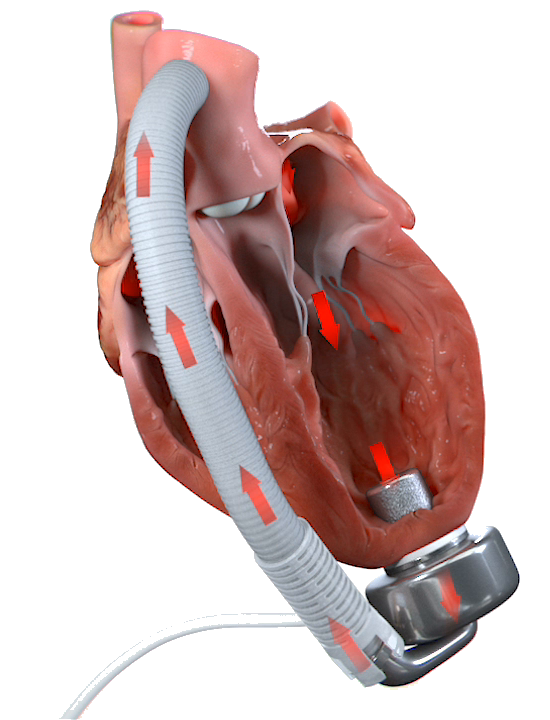
But let‘s take another step back to better understand the context of my application of this numerical technique. In my Ph.D. research, I decided to adopt X-FEM to simulate the complex dynamics occurring in the so-called Wave Membrane Blood Pump, developed at CorWave SA (Clichy, France). Indeed, this novel pumping technology is based on the mutual interaction between the blood flow and an undulating polymer membrane, which results in an effective propulsion working against the adverse pressure gradient between the left ventricle and the aorta. Therefore, we are technically dealing with a 3D Fluid-Structure Interaction (FSI) problem with a thin immersed membrane that undergoes to large displacements. The X-FEM formulation for this challenging class of FSI problems was proposed in [2].

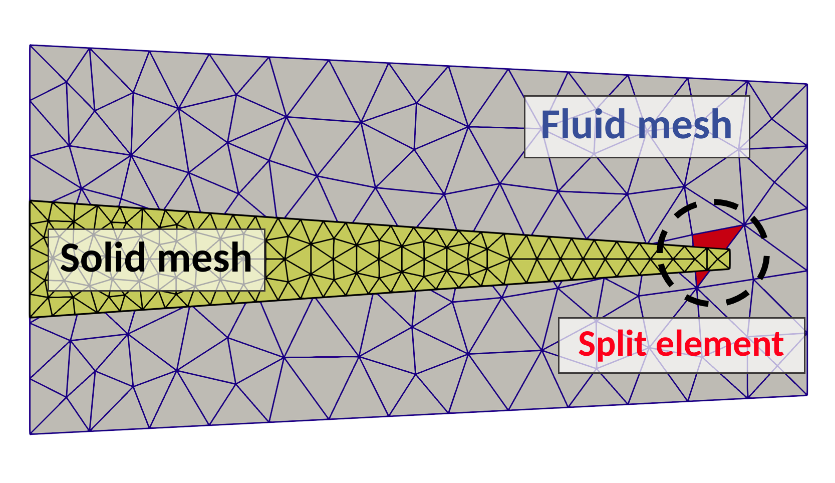
In FSI problems we need at least two meshes, one for the fluid and one for the structure. Since XFEM is an unfitted mesh technique, the two meshes lay on two different levels: in the background, there is the fluid mesh, that is fixed in time; while in the foreground, the structure mesh is free to move and intersect the underlying fluid mesh (see Figure 1). This means that some fluid mesh elements are cut by the structure mesh and perhaps split into multiple parts, where we need to represent the fluid solution. These fluid elements are called split elements. Notice that the split elements change in time because the structure mesh moves and intersects different fluid elements in different ways.

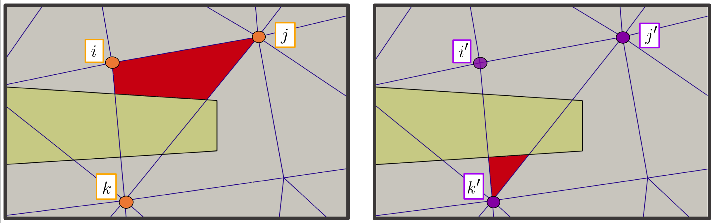
Now, here’s the trick of X-FEM. The split elements are enriched – or extended – by duplicating the corresponding dofs. Hence, we can use a set of dofs (i, j, k) to integrate the solution in one fluid visible portion of the split element, and the second set of dofs (i’, j’, k’) to integrate the solution in the other portion (see Figure 2). In this way, we end up with a simple way to embed a discontinuous solution in the same (extended) finite element using standard basis functions for the integration in space. Otherwise, in FEM framework, we would need to switch to discontinuous modal basis functions directly defined on the polyhedra generated by the intersetion, making the problem very stiff in three dimensions.

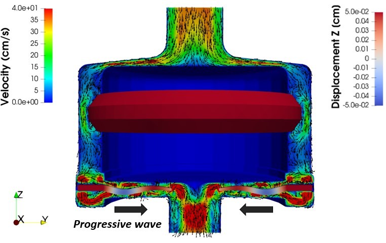
However, I must add that even the implementation of X-FEM is not simple, because we need to compute the intersections between the fluid and the structure meshes at each timestep and duplicate the dofs accordingly. Indeed, to my knowledge, this is the first time that X-FEM is applied on a real 3D industrial problem. Nevertheless, we validated the X-FEM-based numerical model against experimental data, proving that it is a reliable predictive tool for the hydraulic performance of the pump device [3]. In Figure 3, I report a snapshot from an X-FEM simulation of the FSI in the wave membrane blood pump, where we visualize the blood velocity field and the displcament field of the elastic wave membrane.

I hope I have “extended” a bit your knowledge. Sorry for the bad joke.

[1] A. Hansbo and P. Hansbo. An unfitted finite element method, based on Nitsche’s method, for elliptic interface problems. Computer methods in applied mechanics and engineering, 2002

[2] S. Zonca, C. Vergara, and L. Formaggia. An unfitted formulation for the interaction of an incompressible fluid with a thick structure via an XFEM/DG approach. SIAM Journal on Scientific Computing, 2018

[3] M. Martinolli, J. Biasetti, S. Zonca, L. Polverelli, C. Vergara, Extended Finite Element Method for Fluid- Structure Interaction in Wave Membrane Blood Pumps, submitted, MOX-Report 39/2020, 2020

August just ended and we are coming back to our research. But summer is still all around us and the mind easily go back to the last months with vivid memories of sunny days. So, I will take a break from any technicality and will tell you the story of my summer adventure.

It is June and we are finally allowed to get out. Being locked at home for months makes any relationship stiff and rusty. So one of the first thing I want to do is to meet again my dearest friend Paolo. Together we already cycled from Savona (north of Italy) to Lisbon years ago and we know each other so well that in few minutes the familiar feeling is back. Summer is approaching so we go back to the adventures we had together. Soon we get excited and start thinking about possible projects. We have only one week, not too bad but still too little time for great projects. Apparently. Some nice Alps trail, France, the Balkans. The ideas are many. But looking at the maps Paolo spots two points: Bardonecchia – Otranto and a straight line connecting them. The westernmost and the easternmost towns of Italian Peninsula. Already excited, we check the mileage. It is more than 1500km. We have seven days. Here comes the math: it is more than 200km per day. Non of us have ever made 200km in a day. I spot a twinkle in his eyes, the brain is already cycling. We fix the date.

One month later, the 25th of July, we are looking at the sunrise in Bardonecchia with fully packed bikes ready to cycle. From now on, our main thought is “keep pedalling”. The more we cycle, the souther we get. Every day, the accent changes and so the food, the attitude, the landscape. We go so fast through Italy that it is an overdose of sun and beauty.
We organized the trip to visit friends we do not meet since a long time. Then, when we arrive every evening, a friend is waiting for us. They immediately understand how exhausted we are after 10 hours of cycling. Every time, our host is full of care understanding our needs and thought. The feeling is to arrive at home every day.
As the days pass, the fatigue on our body increases, the days get hotter. Now we need to rest at midday because the thermometer goes over 40 degrees. In a single day, we drink over 20 water bottle trying to keep some water in the body. But we do not stop. Now we have crossed the Apennines, the number of kilometers per day increases but there are no more climbs to do. Orientation is not a problem anymore, we follow the sea line. The sixth day, we cycle in the sunshine the trabocchi coast. Every kilometer there is an ancient wood building going over the sea. They were built and used by farmers to fish because they did not know how to sail. I have never seen a clearer water and a more beautiful coast.

Reaching Barletta for the last stay before Otranto, we now we are going to success. We know that soon will be time to celebrate. The last day, we go so fast and happy that we arrive several hours earlier than expected. The town council is waiting for us and we arrive shouting and crying for the joy. The adventure is over. It was the adventure of a ROMSOC fellow.

About the author

Umberto Emil Morelli is an early stage researcher within ROMSOC. He is doing his PhD in reduced order modeling for boundary conditions estimation in heat transfer problems at the Technological Institute for Industrial Mathematics (ITMATI) in collaboration with Danieli & C. Officine Meccaniche SpA and the Scuola Internazionale Superiore di Studi Avanzati (SISSA).

Regardless of the mode, transportation – as an industry –  faces numerous planning challenges, beyond these seen in other industries. They frequently entail thousands of interdependent decisions, with an element of uncertainty. This is why for many years, optimization techniques have found extensive use in that branch of economy. In this post, I would like to present some of the most prominent applications of optimization techniques in transportation, with a particular focus on rail freight transportation. I will also mention some works relating to each of the applications discussed. This choice is due to my own research focusing on that mode of transport.

Let us start from the broad perspective of the railway network of a country. With a history starting in the 19th century, these were frequently built by numerous companies, serving their own interests. Over time, they grew bigger and bigger, and gradually found themselves under the control of one entity, usually a state-owned company which maintains them and sells the access slots (just like at an airport). Now, as the transportation needs change, some of the lines are shut down while others are refurbished. On some occasions, completely new lines are built.

To assist decision-making while considering an extension to a railway network, policy-makers can use tools like those described in Andreas Bärmann’s [1]. Andreas uses forecasts of the demand for access to the railway network at different points in Germany and comes up with a model which highlights the sections of the network which will experience the greatest increase in demand. To make the problem solve efficiently, he inter alia develops a decomposition technique, made to the measure of the studied multi-period network design problem.

Going further, the network manager needs to distribute the access rights to the network. This is required in order to – in the most general terms – maintain safety in the network and assure that as many trains as possible can access the railway line. In particular, a certain distance – called headway – needs to be kept between two consecutive trains. Further, especially on the electrified sections of the network, an appropriate train schedule can help save energy thanks to recuperation.

One of the most prominent papers dealing with the described problem was written by Alberto Caprara, Matteo Fischetti and Paolo Toth [2]. They develop a graph theoretic formulation for the problem of scheduling trains on a single, one-way track linking two major stations, with a number of intermediate stations in between using a directed multigraph. They then use Lagrangian relaxation to arrive at an efficient heuristic solution algorithm, and demonstrate the results on instances supplied by two Italian railway network managers. More recently, my colleagues from the chair, Prof. Alexander Martin, Dr. Andreas Bärmann (who are the supervisors of my thesis) and others [3] together with VAG (transportation authority of Nuremberg metropolitan area) developed an approach to optimal timetabling aiming at minimizing the energy consumption of the trains through more energy-efficient driving as well as by increasing the usability of recuperated energy from braking. This solution could soon be used by VAG in their timetabling process. This work is part of a project on energy-saving via real-time driver assistant systems for interconnected trains in the ADA-Lovelace-Center in Nuremberg, Germany [4]. It is a research centre for artificial itelligence (AI) founded jointly by the Fraunhofer Institute for Integrated Circuits (IIS), the Friedrich-Alexander University Erlangen-Nürnberg (FAU) and the Ludwig-Maximilian University München (LMU) [5]. Its mission is to push methodological advancements in AI and to act as a platform for AI collaboration between research and industry.

Another important application of mathematical optimization pertains to the decisions relating to the production resources of a railway carrier, most important of which are locomotives and drivers. On one hand, one needs to ensure that both an appropriate locomotive (e.g. suitable to the line, powerful enough) and an appropriate driver (e.g. licensed to drive the mentioned locomotive on the train’s route) is attributed to the train, on the other hand, each driver has a number of working time constraints, and locos require maintenance. Other assets considered frequently include wagons and passenger train personnel.

A prominent paper pertaining to locomotive scheduling is the one by Ahuja et al. [6]. They study a problem of assigning locomotive consists to pre-planned trains, aiming at supplying each train with appropriate power. Another one, by Jütte et al. [7], uses column-generation techniques to develop and implement a crew-scheduling system at DB Schenker, the largest European rail freight carrier. My own research focuses on combining both problems (posed differently) into one, and solving them “from one hand”.

All of the abovementioned applications are just the “tip of the iceberg”. In this post, I only covered three macro-stages of planning in the railway industry, and showed how can mathematical optimization be of help there. Other applications could include e.g. train control, locomotive maintenance scheduling, shunting, train dispatch and delay management. Vast majority of those, as well as others, were all described in [8], which should serve as an reference point to the interested reader.

[1] ] Bärmann, A., 2015. Solving Network Design Problems via Decomposition, Aggregation and Approximation. Springer Spektrum. https://doi.org/10.1007/978-3-658-13913-1

[2] Caprara, A., Fischetti, M., Toth, P., 2002. Modeling and Solving the Train Timetabling Problem. Operations Research 50, 851–861. https://doi.org/10.1287/opre.50.5.851.362

[3] Bärmann, A., Gemander, P., Martin, A., Merkert, M., Nöth, F., 2019. Energy-Efficient Timetabling in a German Underground System. Preprint. http://www.optimization-online.org/DB_FILE/2020/04/7728.pdf

[4] https://www.scs.fraunhofer.de/en/focus-projects/ada-center/ai-transport-mobility.html

[5] https://www.scs.fraunhofer.de/en/focus-projects/ada-center.html

[6] Ahuja, R.K., Liu, J., Orlin, J.B., Sharma, D., Shughart, L.A., 2005. Solving Real-Life Locomotive-Scheduling Problems. Transportation Science 39, 503–517. https://doi.org/10.1287/trsc.1050.0115

[7] Jütte, S., Albers, M., Thonemann, U.W., Haase, K., 2011. Optimizing Railway Crew Scheduling at DB Schenker. Interfaces 41, 109–122. https://doi.org/10.1287/inte.1100.0549

[8] Borndörfer, R., Klug, T., Lamorgese, L., Mannino, C., Reuther, M., Schlechte, T. (Eds.), 2018. Handbook of Optimization in the Railway Industry, International Series in Operations Research & Management Science. Springer International Publishing, Cham. https://doi.org/10.1007/978-3-319-72153-8

About the author:

Jonasz Staszek is an early-stage researcher (ESR7) within ROMSOC. He is working with Friedrich-Alexander-Universität Erlangen-Nürnberg in collaboration with DB Cargo Polska on mixed-integer optimization models for an optimal resource allocation and investment for border-crossing transport services in rail traffic.

Building on the previous blog entry we will continue discussing the combination of model order reduction (MOR) and Multirate (MR) time integration, called the reduced order multirate (ROMR) method.

In this post we’ll explore the effectiveness of the ROMR method by applying it to an example circuit. Hence, consider the circuit depicted in Figure 1. This circuit consists of an operational amplifier, two resistors, a diode and a capacitor. The resistor R(T) produces and transports heat and is temperature dependent. The amplifier is a heat source

and the diode has a temperature dependent characteristic curve. Now this system can be naturally partitioned into a slow and fast subsystem by grouping together the electrical equations in a fast subsystem and the discretized thermal equations in a slower subsystem. Furthermore, the large nonlinear thermal subsystem is reduced by a reductive projection matrix, V. The system can then be mathematically described by

where the overdots denote time derivatives, the subscripts F, S stand for the fast and slow timescales and R indicates the reduced state vector of the slow subsystem. In Figure 2 the results of a transient analysis are shown, in which you can see the different time-scales in action.

To assess the performance of the ROMR scheme the obtained voltages at nodes u 3 and u 4 are compared to a highly accurate reference solution. Figure 3 shows this comparison for the single rate ( scheme, the MR scheme and the ROMR scheme. It shows that the reduced order multirate scheme error, the left figure, follows the O(H) convergence rate. In the right figure, it shows the computation time versus the difference with the

reference solution. From these figures we see that the ROMR scheme decreases the computation time whilst maintaining the MR accuracy. I hope you enjoyed this instalment of our ROMSOC blog. To follow the progress of my fellow researchers and I please keep an eye on the ROMSOC website and follow us on Twitter and Facebook!

For now servus and a rrivederci
Marcus Bannenberg

About the author

Marcus Bannenberg is an early stage researcher ( in the Reduced Order Modeling Simulation Optimization and Coupled methods ( project. He is a PhD student at the Bergische Universität Wuppertal and working in collaboration with STMicroelectronics. His research project is focus ed in numerical analysis/applied mathematics on the combination of model order reduction and multirate techniques.

In my last blog post , we got an overview on the origins of sound while highlighting the motivations for the ESR02 subproject within ROMSOC. (TLDR : Its to develop coupled mathematical models to compute the influence of turbulent fluid and porous media on a sound measurements). This time around we focus on simplifying the scope and complexities accounted in a target mathematical model for sound measurements. Measuring sound provides valuable insights in engineering tasks. The knowledge of acoustic characteristics of materials and structures obtained apriori is valuable to designers and architects. Measurements are also necessary to enhance user experience in loudspeakers etc. In product maintenance and diagnostics, e.g of a vehicle, sound signal provides information on health and performance, and is constantly monitored. But how are these measurements performed? Typically, a simplified measurement procedure involves, a receiver, (or sensor) which captures the sound signal. Receivers come with different accuracy, sensitivity and range in sound level measurements. It is also packaged differently to suit the environment. Knowing the measurement environment is extremely important, since enclosures cause reflections of incident sound signals and also induce it’s own resonance. External noise may also deter accuracy and in some cases, there also are chambers designed specifically to prevent external noise from impacting measurements (anechoic chambers). Information about sound source is also to be taken into account. A distribution of sources, e.g a set of loudspeakers can have interference patterns, while a moving source (relative to the receiver) exhibits a shift in frequencies, known as the Doppler effect.

Recreating such an entire procedure on a computer involves replicating the entire setupdigitally – making it necessary to encode the physical process into mathematical equations. The French mathematician, Jean D’Alembert (1717-1783) is credited with arriving at the concise equation describing the motion of a sound wave (in 1D) through a medium,

The wave equation is a well-known partial differential equation and is of great importance in various applications. The equation has multiple solutions most of which maybe physically unfeasible and need additional information from the domain of interest to completely describe the motion of sound. This is where models for sound sources and environmental conditions are factored. The image below illustrates the generation of a spherical wave from a point-sized source at the center of the rectangular domain.

While the wave propagation model above explains the sound propagation in sparsemedium like air, it is complex in porous layer media. Models on acoustical behavior in porous materials were presented only in the 1950s by Zwikker, Kosten and Biot followed until the present by more detailed models. Sound transmission through porous materials are distorted severely influenced by the porous micro-structures and the fractional volume of the air. It is being subjected to viscous and thermal resistances, while also being deferentially transmitted through the fluid within the media and the porous frame. A detailed acoustical model replicating their effects need to consider the macroscopic effects on an incident signal and the choice of the right model depends on the type of porous material in a specific application.

Physical processes in the nature are often observed as a multitude of phenomena happening simultaneously and need simplification to quantify, analyze and predict them. A variety of models need to be sewn together to reproduce the phenomena in a computer accurately. The ROMSOC project aims to address this very issue through mathematical modeling and coupling. Follow our project blog for more posts in the topic.

About the author:
Ashwin Nayak is an early-stage researcher (ESR2) in the Reduced Order Modeling Simulation Optimization and Coupled methods (ROMSOC) project. He is affiliated with the Technological Institute of Industrial Mathematics (ITMATI), Spain and working in collaboration with Microflown Technologies B.V., Netherlands. His research aims to develop coupled mathematical models to enable acoustical measurements in fluidporous
media interactions.

2020 started recently so it’s time to look into the stars again. I will continue with my last year’s blog post “A new year has started. Let’s look into the stars!” and share with you my current challenges at work that are all about “How fast can we get for the European Extremely Large Telescope?”

As already described in my first blog post, my research is dealing with adaptive optics and, in particular, with the problem of atmospheric tomography for the European Extremely Large Telescope (ELT). Because the atmosphere is changing rapidly this problem has to be solved in real-time. In our case, real-time means within two milliseconds. These requirement is quite challenging for the ELT, because the telescope is large which leads to a huge amount of data that has to be processed. The challenge I’m dealing with is how to optimize the performance of solving the atmospheric tomography problem.
The first decision you have to make when dealing with performance optimizations is which algorithm you want to use. Within my research, I have to solve a system of equations which is a common problem in many real world applications. You can either choose a direct solver or an iterative one. In contrast to the direct solver, an iterative approach starts with an initial guess and iterates until it reaches a solution that is good enough. In general, iterative solvers are better for very large and sparse systems. Moreover, you have the possibility to use an iterative solver in a matrix-free fashion, i.e., avoid to store all the matrix entries which saves a lot of memory.
If you want to improve the performance of an existing algorithm you usually try to parallelize, i.e., execute steps in parallel. For example, when adding two vectors of length n every entry is completely independent from the others. Thus, you can execute the n additions in parallel and save a lot of time. For more complex algorithms deciding where and how to parallelize becomes a quite challenging task.
Another non-negligible aspect is the right hardware. A topic in which mathematicians are in general not well versed. This is one of the nice things about ROMSOC. Half of my PhD I’m working at the company Microgate with specialists in real-time hardware. This gives me the possibility to look into various fields, not only mathematics, and improve my interdisciplinary skills. At the moment we are running our algorithm on the high end GPU NVIDIA Tesla V100 at Microgate as well as on a high performance computing cluster called Radon1 from RICAM in Linz.

• 

• 

Altogether, performance optimization is a hard task. You never know in advance if you can gain enough speed for your underlying algorithm which can become quit gruelling after a while. Nevertheless, it is something really important for practical applications and something many mathematicians do not pay enough attention.

About the author

Bernadett Stadler studied Industrial Mathematics at the Johannes Kepler University in Linz. Since May 2018 she is part of the ROMSOC program as a PhD student. She is involved in a cooperation of the university in Linz and the company Microgate in Bolzano. Her research addresses the improvement of the image quality of extremely large telescopes. The goal is to enable a sharper view of more distant celestial objects.

Port-Hamiltonian systems are network-based models that are formed by decomposing a physical system into submodels that are interconnected via energy exchange. The submodles may arise from different physical domains, such as e.g. electrical, thermodynamic, or mechanical systems.   The  port-Hamiltonian structure is preserved under power conserving interconnection, and properties stability, passivity, as well as conservation of energy and momentum are encoded directly into the structure of the model.

When the  Interconnection of submodels leads to further constraints such  as Kirchoff’s laws or position and velocity constraints  in mechanical systems, then the appropriate model class is that of port-Hamiltonian descriptor systems. In the last year model reduction techniques for port-Hamiltonian descriptor systems have received substantial attention and major progress has been made in substantially reducing the model dimensions while fully preserving the constraints.  This has a major impact on the use of these models in practice. While the dimension of the dynamical part can be drastically reduced, the constraints are still valid, so a replacement of the full model by a reduced model in any  subcomponent will not violate the underlying physics and thus each subcomponent can be modelled as a modl hierarchy where depending on the application a detailed or a coarse model is used.

See the recent papers

C.A. Beattie, S. Gugercin and V. Mehrmann, Structure-preserving Interpolatory Model Reduction
for Port-Hamiltonian Differential-Algebraic Systems. http://arxiv.org/abs/1910.05674, 2019.

S. Hauschild, N. Marheineke, and V. Mehrmann,
Model reduction techniques for linear constant coefficient port-Hamiltonian differential-algebraic systems,
https://arxiv.org/abs/1901.10242, 2019. To appear in ‘Control and Cybernetics’.

For examples of controlled flow problems or mechanical multi-body systems.

About the author:
Professor Dr. Volker Mehrmann is full professor for Mathematics at Technische Universität Berlin and the president of the European Mathematical Society (EMS). Moreover, he is the coordinator of the ROMSOC project.

Alongside his activities for the EMS, he has been sitting on the boards of the International Council for Industrial and Applied Mathematics (ICIAM) and the EU-MATHS-IN initiative, which promotes collaboration between mathematics researchers and industry. Additionally he is a member of the German Academy of Science and Engineering (acatech) and acted as spokesperson for the Berlin research center for application driven mathematics MATHEON between 2008 and 2016.

He can look back on many years of active commitment to international exchange and the promotion of mathematics and its applications and seeks to improve communication and cooperation between mathematical disciplines as well as between mathematics and other sciences focusing also on the promotion of early-career researchers and women in mathematics.

His research interests are in the areas of numerical mathematics/scientific computing, applied and numerical linear algebra, control theory, and the theory and numerical solution of differential-algebraic equations. In recent years he focuses on the modelling, simulation and control of systems described by port-Hamiltonian differential-algebraic systems, which form an exciting and very promising new modeling paradigm.

Steel making is a very old process and has contributed to development of technological societies since ancient times. The previous stage to steelmaking is the ironmaking process, which is performed inside blast furnace. Blast furnace is a metallurgical reactor used to produce hot metal (95% Fe, 4.5%C) from iron ore. The burden contains iron ore, fluxes and coke. The process involves an exothermic reaction, the gasification of carbon. High temperature inside the blast furnace is required to increase the gasification of carbon. The temperature in the hearth can be as high as 1500 degree Celsius. The thermal stresses induced by high temperature inside the blast furnace hearth limit the overall blast furnace campaign period. The numerical computation of thermal stresses requires coupling of thermal and mechanical models and solve the associated coupled system.

My work in this project has two main objectives. First objective is to numerically compute temperature profile inside the blast furnace hearth walls and compute thermal stresses. This requires application of concepts from the field of continuum mechanics, numerical analysis and scientific computing. However, the increasing demand of these fields for complex processes has put computational resources under considerable pressure. This is particularly true if such computations are required to be performed repeatedly at different parameters. By parameters, we mean variations in the material properties or in the geometry of the domain of interest. In the absence of efficient computational algorithms, the simulations might be time consuming, if not unfeasible, with available computational power. Hence, another objective of my work is to make the computations faster and efficient while maintaining reliability of numerical simulation above minimum acceptable level by using techniques of reduced order modeling for parametric partial differential equations.

Interdisciplinary nature of this project brings additional challenges. While working with the industrial partner, inputs about the processes from experienced professionals in the field of blast furnace operations and experimental measurements are gathered. During the analysis work, mathematical methodologies are devised under supervision of experts in the field of continuum mechanics, applied mathematics and scientific computing. It can be quite challenging sometimes to coordinate and bring everyone at the common platform. This challenge has motivated me to develop skills in various fields in order to be capable of working with experts from different domains. Besides, an industrial doctorate in the ROMSOC project framework has provided me environment to be disciplined as a professional as well as flexible and open minded as a researcher. In addition to the skills obtained within an individual project, the training courses and networking opportunities have contributed significantly by providing overview of concepts in other potentially relevant areas and in turn, have helped to gain alternative perspective about research.

I am confident that the learning process will continue further and I look forward to positively contribute to the organizations involved and at large, to the scientific community.

About the author:

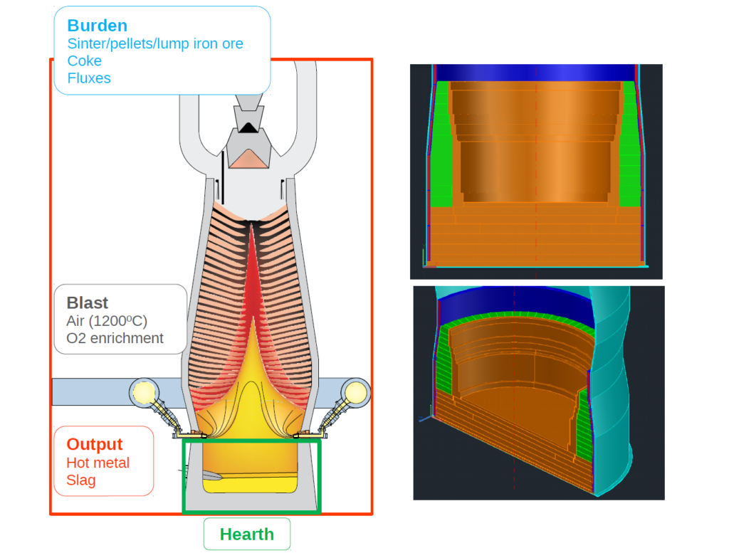
Nirav Vasant Shah is an Early-Stage Researcher (ESR10) within the ROMSOC project. He is a PhD student at the Scuola Internazionale Superiore di Studi Avanzati di Trieste (SISSA) in Trieste (Italy). He is working in collaboration with ArcelorMittal, the world’s leading steel and mining company, in Asturias (Spain) and Technological Institute for Industrial Mathematics (ITMATI) in Santiago de Compostela (Spain) on the mathematical modelling of thermo-mechanical phenomena arising in blast furnace hearth with application of model reduction techniques.”

by Marco Martinolli

My story as a Marie Sklodowska-Curie Action (MSCA) Fellow started on March 2018. It has been 1 year and a half full of experiences, travels and hard work, that made me grow both professionally and personally in many ways. Therefore, being at the midway of my Ph.D. carreer at Politecnico di Milano (Milan, Italy), it is a good moment to look back and make some considerations of my experience as ESR9 within ROMSOC doctoral project.

In this time, I have had the opportunity to work on an industrial project with a mission in which I deeply believe: improve the life conditions of people affected by advanced heart failure. In fact, my research topic consists in the numerical study of membrane-based blood pumps, which are implantable devices that support the cardiac function of damaged hearts. Specifically, I study the fluid-structure interaction that arises in a novel prototype of blood pumps developed at CorWave Inc. (Paris, France). In these pump systems, the propelling action of an oscillating elastic membrane results in the ejection of blood from the left ventricle into the aorta in a pulsatile regime. My goal is to model the membrane-blood dynamics and simulate the pump system in three-dimensions, so that it is possible to predict the hydraulic performance of the pump and optimize it under different operative conditions. As a mathematical engineer, it makes me proud to employ my numerical and computational skills on a real application with potential beneficial effects on the global health system.

Besides my research activity, my job as a MSCA Fellow includes many other tasks and responsibilities, going from the participation to an European training program in advanced mathematics to the creation of teaching material for other students in the field of coupling methods. In particular, in the last months I have worked a lot for the organization of an upcoming scientific event, the Workshop of Industrial Mathematics (WIM2019) in Strobl, Austria. This type of commitment was new for me and allowed me to enhance my abilities in managing resources and coordinating people.

An important mission of my doctoral program is also research dissemination. For this reason, I attended to several important congresses and conferences, like INDAM2018 in Rome, ESAO2018 in Madrid or ICIAM2019 in Valencia, to study cutting-edge technologies and promote my research. But the experience that taught me the most is actually my recent participation to the European Researchers’ Night, a scientific event organized within the Horizon2020 program that is aimed at involving the general public in the activities of the local scientific realities. Participating at the MEETmeTONIGHT exhibition in Milan on September 27th allowed me for the first time to present my research to people with different ages and backgrounds. I had the pleasure to entertain young students from high schools as well as families with kids using science and mathematics and I have learnt how to adjust my communication style depending on the audience.

Finally, this experience has encountered my international aspirations. In fact, in order to work at the partner company, I have lived in Paris – a city that I love – for 6 months and I am about to move there again for another year. This job gave me also the chance to travel around Spain, France, Germany and Austria, expanding my linguistic knowledge and my relational skills in multi-cultural and multi-ethnical communities.

To be honest, the path through my European doctorate has not been always easy and smooth: I have experienced the different approaches of the academic and industrial environments and consequently the different expectations that they have from my work; I have had to manage my time between the progress on my research and the deliverables for the ROMSOC project; and, not to be underestimated, I also struggled to find an accommodation every 6 months in Milan and Paris. However, I strongly believe that all the challenges faced in these first 1.5 years made me a better worker under many points of view and that my future carreer will benefit a lot of this personal and professional growth. Plus, I will bring with me also many good memories.

Marco Martinolli is an Early-Stage Researcher (ESR9) within the ROMSOC project. He is a PhD student at Politecnico di Milano (Milan, Italy) and is working in collaboration with CorWave Inc. (Paris, France). His research project deals with numerical simulations for the fluid-structure interaction arising in blood pumps based on wave membranes.

References:

[1] A. Binder, O. Jadhav, and V. Mehrmann. Model order reduction for parametric high dimensional models in the analysis of financial risk. Technical report, 2020. https://arXiv:2002.11976.