Blog

Most of the steel we use every day comes from continuous casting. This is a process which was first introduced in the 1950s, but the first patents are hundred years older. Before continuous casting, the steel was poured into closed molds to form ingots. With the development of continuous caster became possible to produce continuous billet, blooms or slabs. It allowed to have very long pieces with better quality, much faster. The thecnology has improved since its invevention and nowadays these casters can produce up to 10 meters of steel per minute.

The industrial partner of this project is the Italian steelmaking company Danieli & C. Officine Meccaniche SpA, they design and run continuous casters. According to the ROMSOC DNA, Danieli came up with the challenge. As these casters go faster and faster, to control the quality of the product becomes harder and harder. The main problems arise in the mold. There the steel begins its solidification and external imperfections can appear due to a wrong heat extraction from the mold which is cooling down the steel.

Until now, steelmakers used thermocouples to measure the temperature at some points in the mold. This in not sufficient for a proper understanding of the behavior of the mold because what we are really interested in is the heat flux between the mold an the solidifying steel. Then, the objective of my project is to develop a method for estimating the heat flux at the boundary of the mold based on the measurements of the thermocouples made inside the mold domain. Moreover, this has to be done in real time. This problem is what we call an inverse problem. As you may know, it ain’t easy to work with inverse problems which, by the way, are ill-posed. Several techniques are available for solving this kind of problem however they are generally computationally expensive. Here is where Model Order Reduction (MOR) comes into the picture. In my project, we want to exploit MOR to speed up the solution of this inverse heat transfer problem obtaining real time computations of the heat flux. After this brief overview of the subject of my PhD, in the next posts I will go deeper in the methodology we are developing. So keep visiting the ROMSOC blog to stay updated with mine and all other terrific projects.

About the author

Umberto Emil Morelli is an early stage researcher within ROMSOC. He is doing his PhD in reduced order modeling for boundary conditions estimation in heat transfer problems at the Technological Institute for Industrial Mathematics (ITMATI) in collaboration with Danieli & C. Officine Meccaniche SpA and the Scuola Internazionale Superiore di Studi Avanzati (SISSA).

Between 22nd and 26th of July of this year, (almost) all of the ESRs of the ROMSOC Program took part in the Mandatory Training Course in Mathematical Optimization at University of Erlangen–Nuremberg.

During that time, we have received a thorough introduction to mathematical optimization as such. We learned about the challenges with regard to integer programming. We also practiced solving such problems, both by hand and using state-of-the-art software (Gurobi). Differences between good and bad model formulations were discussed as well.

We also held numerous exchanges about the applications of the mathematical optimization, particularly on the planning problems in industry. We learned how to build optimization models which are applicable to problems occurring in logistics and transport, as well as production, energy systems, telecommunications and many more. We also had a long discussion about the use of optimization in the context of social equity vs. efficiency.

Finally, we went for an excursion into the Franconian mountains, where – despite unfavorable weather – we had a chance to discuss our views and ideas on the subject in an informal setting.

The course was led by professor H. Paul Williams – a person of paramount importance in the world of discrete optimization. We had a chance to benefit from his decade-long experience in the field, starting from the professor’s first attempt to formulate a production model in 1960s, when punched cards were still required to run any kind of computer, through the times when he worked at IBM to develop one of the first optimization software packages (MSPX), and ending in academia, ultimately at LSE.

Below are some pictures from the event:

 

About the author:

Jonasz Staszek is an early-stage researcher (ESR7) within ROMSOC. He is working with Friedrich-Alexander-Universität Erlangen-Nürnberg in collaboration with DB Cargo Polska on mixed-integer optimization models for an optimal resource allocation and investment for border-crossing transport services in rail traffic.

 

There I was considering my options after graduation. Different thoughts were rambling across my mind, the idea of getting an advanced degree like Ph.D., and learning a topic at a deeper level intrigued me. I truly enjoyed working on my master thesis and decided to pursue my Ph.D. in the same field.
So, what do I do? Ah, the question that triggers an existential crisis. Sometimes, this comes from innocent, friendly strangers who are trying to spark a conversation. This image from the ‘PhDcomics’ really justifies the length of time it takes you to answer the question “So, what do you do?” Hmm… Let me try to explain it. Just hang in there, you are bound to understand one of the modern problems in the financial mathematics and my humble efforts to solve it.

Problem:

Packaged retail investment and insurance products (PRIIPs) are at the essence of the retail investment market. PRIIPs offer considerable benefits for retail investors which make up a market in Europe worth up to € 10 trillion. However, the product information provided by financial institutions to investors can be overly complicated and contains confusing legalese. To overcome these shortcomings, the EU has introduced new regulations on PRIIPs (European Parliament Regulation (EU) No 1286/2014). According to this regulation, a PRIIP manufacturer must provide a key information document (KID) for an underlying product that is easy to read and understand. The PRIIPs include the interest rate derivatives such as floating coupon bonds, or interest rates cap and floors.

A KID includes a section about ‘what could an investor get in return?’ for the invested product’ which requires costly numerical simulations of financial instruments. Generally, the interest rate derivatives are evaluated based on the dynamics of the short-rate models. For the simulations of short-rate models, techniques based on discretized convection-diffusion reaction partial differential equations (PDEs) are often superior. It is necessary to note that the choice of a short rate model depends on the type of financial instrument. The Hull-White model is one of the examples of the short rate models:

The model parameters are usually calibrated based on market structures like yield curves. A yield curve shows the interest rates varying with respect to the 20-30 time points known as ‘Tenor points’.

Current idea:

So, in short, the goal is to reduce the computational complexity in the analysis of financial instruments. To avoid this problem, we are working on a parametric model order reduction (MOR) approach based on the proper orthogonal decomposition (POD) method. The method is also known as the Karhunen-Loève decomposition or principal component analysis in statistics. This research work aims to develop a MOR methodology regardless of any short rate model. The technique of model order reduction reduces not only the computational complexity but also the computational time. POD generates an optimally ordered orthonormal basis in the least squares sense for a given set of computational data. Further, the reduced order models are obtained by projecting a high dimensional system onto a low dimensional subspace obtained by truncating the optimal basis. The selection of the computational data set plays an important role, and most prominently obtained by the method of snapshots. In this method, the optimal basis is computed based on the set of state solutions. These state solutions are known as snapshots and are calculated by solving the full model obtained by discretizing the PDE for some parameter values.

The calibration based on simulated yield curves leads to the size of  parameter space. Each parameter vector  has values ranging from   to  , where   is the total number of tenor points and . We compute the snapshot matrix for some selected values of parameters (i.e., snapshots taken at some nodes  ).

The process of computing the optimal basis independent of such a high dimensional parameter space is complex. We aim to develop a new algorithm to obtain the optimal basis based on tensor numerics. We construct a snapshot tensor comprises of the snapshot matrices obtained for certain parameter vectors. Furthermore, we factorize the snapshot tensor using the tensor decomposition techniques to generate the optimal basis. We will then use this optimal subspace for obtaining a parameter-independent reduced order model.

We have implemented the classical POD approach for a numerical example of a puttable bond solved using a Hull-White model. The current research findings indicate that the MOR approach works well for the short rate models and provides two to three times computational speedup (see Fig. 2).

About the author:

Onkar Sandip Jadhav is an early-stage researcher (ESR6) in the ROMSOC project. He is a PhD student at the Technische Universität Berlin (Germany) and is working in collaboration with MathConsult GmbH (Austria). In his research he is working on a parametric model order reduction (MOR) approach aiming to develop a new MOR methodology for high-dimensional convection-diffusion reaction PDEs arising in computational finance with the goal to reduce the computational complexity in the analysis of financial instruments.

As ESR-5 in the ROMSOC project I work at the Bergische Universität Wuppertal (Germany) in the picturesque surroundings of das Bergisches Land and at ST Microelectronics at the foot of Mount Etna in Catania (Italy). After having spent my first three months in Wuppertal, I am now living in Catania for six months. In a stark contrast to the colossal size of the ever looming mount Etna, my research takes me into the miniature world of nanoelectronics.

Microchip details are in the order of meters, one millionth of a millimetre. On that scale a human hair looks like a giant tree. Now many phenomena (electro mechanical, thermal, quantum physical) occur inside microchips. In this blog I will focus on thermal aspects. Given the nano-scale of the details it is impossible to perform any measurements inside a working microchip. To understand and try to improve processes inside microchips we convert them into mathematical equations and apply a combination of multirate (MR) and model order reduction (MOR) techniques. Both techniques are well known individually but combining them is novel.

Our goal is to build a simulation of what happens inside a working microchip to help microchip designers create better products.

The Problem: Simulating A Large Coupled System

In the simulation of nanoelectronics there are a great many things to consider. Whilst trying to accurately model the natural phenomena happening inside a microchip one should also safeguard the feasibility of this models numerical solutions. The focus of this project lies on the simulation of large coupled systems with dierent intrinsic time scales.

So let us start at the beginning and look at the origins of these large coupled systems. A microchip is essentially a circuit of many different components, e.g. resistors or transistors, that interact with each other. These interactions are modelled by means of equations and together they form a system of equations. The equations governing the heat of components and the circuit are coupled together, resulting in a coupled system of equations:

Where is the state vector of the coupled system,  the input and the output vector. Furthermore, we consider the system, the input and the output to be linear for now.
As these circuits get more and more intricate these systems continue to grow in size. For modern day microchips these systems can consist of millions of equations. As one could imagine this would become quite unfeasible for straightforward simulation.

MR and MOR

The objective of this project is to combine MR and MOR to drastically improve the simulation speed. MR can exploit the dierent dynamical time scales of subsystems to improve the overall computational efficiency, without losing the global solution accuracy. MOR aims to reduce the size of subsystems and decrease the numerical effort for each time step whilst maintaining a certain level of accuracy.

MR

Consider the previously mentioned system of circuit equations and heat equations, combined in one generalised system.

with . Since two phenomena act on separate time scales, (circuit equations evolve very fast compared to the slow heat equations) the system can be naturally split into two systems.

Where denote the fast changing, active components and
 the slow changing, latent components of . By using a multirate method this system can be integrated using a macro time step for the latent subsystem and a micro time step for the active subsystem, as illustrated in the figure below.

So MR divides the system into subsystems with different dynamic scales. This results in subsystems with similar intrinsic characteristics, which makes them suitable for model order reduction.

MOR

In MOR the goal is to try to approximate the output  of a large system  of  equations. This approximation is done by creating a smaller system of  equations. This smaller system   should be constructed in such a way that the difference between its output,  and the original, , is small, while is also much smaller than .

In the context of circuit simulation this smaller system is used to obtain faster simulations with results that approximate the full simulation to a certain degree of accuracy. A general form of MOR can be described by choosing suitable matrices and , with  and biorthonormal, to create the following projection:

Which can be expressed in mathematical form by

The Solution: Combining MR and MOR

To give an intuitive example of how to combine these two techniques consider a multirate system as defined by

Note that  is considered to be a linear. Now we can apply model order reduction to    by constructing matrices and . This results in the system

For now this simple example serves as an apt illustration. However, as the dimension of the output variable  is still equal to the dimension of the coupling interface we are not quite there yet, but those technicalities will be a story for another blog post.

The Research Project

The main objective of this project is to combine MR and MOR in an industrial setting. This means that instead of the simple linear system given as an example, more complex systems will be considered, e.g. non-linear time-dependent systems or combinations of a variety of different subsystems linked together for which different types of MR and MOR techniques need to be considered.

Besides the combination of the two techniques other goals include: defining error estimates linked to the accuracy requirements of the iteration level of the optimisation flow, the preservation of overall properties of the system and stability of the dynamic iteration process.

I hope that this brief introduction to my research topic has given you some insight into my daily activities. To follow the progress of my fellow researchers and me please keep a sharp eye on the ROMSOC website and follow us on Twitter and Facebook!
For now tschüss and arrivederci.
Marcus Bannenberg

One of the main purposes of scientific research is to structure the world around us, discovering patterns that transcend and that consequently help to unify applications in various contexts.

In this occasion I would like to show a generic model that has many practical applications, as varied as design of excavation operations, strategies to eliminate military objectives, and selection of projects in companies to obtain greater profits.

A specific case could be the following: frequently most companies have to face equilibrium actions on the realization of certain projects that produce profits and the necessary expenses for carrying out support activities for these projects. Let us suppose that a telecommunications company is evaluating the pros and cons of a project to offer some type of high-speed access service to its customers in the home. The market research shows that this service would produce a good amount of profits, but that they have to be weighed against the cost of carrying out some preliminary projects necessary to make the service possible, for example, increase the fiber optic capacity in the core of the network and the purchase of a new generation of high-speed routers.

What makes these kinds of complicated decisions is that they interact in complex ways: in isolation, the high-speed service gain may not be enough to justify the modernization of the routers; However, once the company has modernized the routers it may be in a position to offer another lucrative project to offer to its customers, and perhaps this new project will tilt the profits in favor of the company. In addition, these interactions can be concatenated: the new project may require other expenses but this may lead to the possibility of other lucrative projects.

In the end, the question would be which projects to devote to and which ones to ignore? It is a simple matter of balancing the costs of realization with the profit opportunities that would be possible.

One way to model these types of decisions is as follows:

There is an underlying set of  projects, where each project    has an associated income   which can be positive or negative. Some projects are prerequisite for the realization of other projects. It may be that a project has more than one prerequisite or possibly none. In addition, a project can be a prerequisite for multiple projects. We will say that a set of  projects is feasible if the prerequisites of any project in   are also in the set. A problem to solve would be to find a feasible set of projects with the highest income.

In terms of graph theory we could define this set with the name of closure: A closure in a directed graph  is a subset of vertices without output arcs, that is, a subset  such that if   and  then .

If we assign a weight  (of arbitrary sign) to each node  of , the problem that concerns us is: find a closure  with the greatest possible weight.

In general, our mission would be to partition the set of vertices into two sets  and , the set closure and its complement. The way in which we will model this problem will be a minimum cut in a certain graph. But in which graph? And how to transform negative weights into positive capabilities for the flow algorithm?

To solve these questions we begin by defining a new graph  , formed by adding a source   and a sink   to . For every vertex  with  let’s add an arc  with capacity , and in the same way for every vertex  with    let’s add an arc  with capacity . We will define the capabilities of the arcs in  later. We can see that the capacity of the cut  is ,  so the value of the maximum flow is at most  .

We would like to guarantee that if   is a minimum cut in this graph, then  is a closure. The way we will achieve this is by defining the capacity of each arc in  as  . Then we can formally define the network in question as:

Surprisingly, it is possible to demonstrate that there is a bijection between the minimum cuts in this graph and the closures in . So it would only be necessary to know an algorithm to find minimum cuts in a graph to solve the problem that concerns us.

This example is one of the most unexpected applications of the theory of flows that occur in daily life and one of my favorites, which shows us how often we can find mathematical models in the most unexpected places. I hope that this small example have been interesting for all of you. Continue following our blog.

About the author:
José Carlos Gutiérrez Pérez from Cuba is an early-stage researcher (ESR4) within the ROMSOC project. He is working at the University of Bremen (Germany) in collaboration with the industrial partner SagivTech (Israel) on the development of new concepts for data-driven approaches, based on neural networks and deep learning,  for model adaptions under efficiency constraints  with applications in Magnetic particle imaging (MPI) technology.

Even though STEM fields have a reputation of dealing with hard problems that are complicated to understand for someone not working in the field, there are lots of examples, where an unsolved problem is simple enough to be explained at middle school level, for example moving sofa problem, or famous Fermat’s conjecture, that was solved only recently, after being open for centuries. Looking at them, one might ask, how simple can a hard problem be? Can it be so simple, that even child in kindergarten can understand? What about so simple, that even kindergartener can come up with? Most kids like shiny objects. So imagine little girl, about 5, playing in room with several rotating mirrors, marbles and so on. It will not take a while until she starts playing with reflections, either using sun, if the room is bright, or maybe a flash-light if there is one. At first she is playing by reflecting light trough several mirrors, maybe making a vampire face as well, if the room is dark enough, then she moves on marbles and their light on the wall. She will soon start detecting how changing the direction of the flash-light, or changing a position of marbles and mirrors changes light on the wall. And if she will not be disturbed, she will ultimately come up with a question, on which many scientists have spent lot’s of time, on which many PhD theses were written and answer of which worth millions for big companies, but is still an open problem in most cases:

“How should I arrange those things, to get exactly the shape of light I want on the wall?”

One might wonder, what makes this question so hard to answer. After all, reflection rules are taught in middle school physics, why is it hard to to figure out the shape on which this rule should be applied to? In fact, there are simple abstract models, where equations for a mirror are derived from those rules, but those models are quite far from most applications, and even then, having equation does not guarantee to have a good way of solving it. For example, two simplest and relatively well studied models are “Collimated source” and “Point-source”. The Collimated source model assumes that all light rays are parallel and hit the mirror from the same direction (it tries to mimic sun light, but disregards all the refraction happening in atmosphere, so in practice it is good only for some high-tech lasers).

The Point-source model assumes that all light comes from same point (it is a bit closer to realsituations, think about a flash-light, but with really, really small lightbulb).

In those models, a shape of the reflector can be computed from solution of following partial differential equation:

As most mathematical equations, this one looks scary for someone who does not understand what it means, but it is a rare exception in the sense that this equation looks even scarier for those who understand: It is a fully non-linear Monge-Ampere type partial differential equation. For those who don’t know: it means that all classical ways of solving PDEs fail miserably for this one.

Here for the rescue comes Optimal Transport, the theory that originated from the problem which is again very simple to explain, but hard enough, that it has been around for more than two centuries without much progress. Until a couple of decades ago, when it found it’s second breathe and developed into one of the fastest growing mathematical fields: Given an initial distribution of resources, for example bakeries in Paris which produce some amount of fresh croissants every morning, a desired allocation of those resources, for example cafeterias which need some amount of croissants every morning, and a known cost of transporting those croissants from each bakery to each cafeteria, what is the optimal arrangement of transporting those resources, with respect to the total cost, or in other words, how to decide which cafeterias should each bakery supply, in order to minimize the total cost of transporting all
croissants.

This theory has found its way through both fundamental and applied mathematics, physics, natural sciences, economics and technology, providing new developments as well as refreshed views on existing subjects. For above-mentioned optics problems, it provided a new description of same models, which gave them access to all the fruits of Optimal Transport theory, including robust tools for finding solutions.

But even then, there are still lots of simple questions in that small part of optics, that are left open even after using Optimal Transport. For example, what if the light source is not a point, but something bigger? What if there is more then one mirror? So maybe, we should also be asking: How hard can a simple problem be?

 

 

About the author:
Giorgi Rukhaia is an early-stage researcher (ESR3) in the ROMSOC project. He is affiliated with the Institut national de recherche en informatique et en automatique (INRIA) in Paris, France and working in collaboration with Signify (former Philips Lighting), the Netherlands. In his research project he is working  on an Optimal Transportation computational approach and the development of numerical algorithms for the inverse free-form optical surfaces design using extended sources.

Sound is a physical phenomenon of much prominence in human life considering each of us has a pair of dedicated sensors (ears) to perceiving it. Be it in communication, in music, structural design – the knowledge of how sound works is of extreme relevance.

Acoustics, the science of sound evolved as one of the most interdisciplinary fields drawing inputs from various disciplines like music, architecture, engineering, biology and medicine etc. As such, while having no dearth of literature in the topic, it can be hard to find ground amidst all the perspectives out there. In this article, I focus on my perspectives on the origins of acoustics and its relevance in my project. As for the outcome, I hope to communicate the motivation of my project – to develop better acoustic models enabling more accurate measurements of sound.

The origin of sound is identified to be perturbations in pressure and this is physically caused bydifferent processes – due to vibrating bodies, rapid change in fluid flow, pulsating thermal sources, shocks etc. The theory of sound began as study of vibrations in acoustic instruments and gradually integrated the principles from the theory of mechanics and waves in the 17-18th century. The 19th century made significant leaps in the development of acoustic theory, establishing the mathematics of acoustics – of particular mention, “Theory of Sound”, the classical two-volume treatise by Lord Rayleigh. The theory has since, branched and developed into various disciplines viz. architectural acoustics, aeroacoustics, thermoacoustics, psychoacoustics among others. The 20th century with the development of Modern Physics and improved engineering has improved our understanding andability to control the acoustics.

Let us take deep dive into the process of sound wave transmission. Sounds, being physical perturbations, cannot travel in vacuum and needs a medium to be transmitted. The transmission process is different depending on the nature of the medium i.e. a rigid solid or fluid – characterized by their inter-molecular spacing and structure. Sound transmission are also dependent on thermodynamic properties of the media like pressure (for fluids), density, temperature and also on their elastic properties characterizing their ability to resist perturbations. Furthermore, any phenomenon which alters the above properties need to be considered. Besides these stereotypical classifications of the media, special materials like semi-solids, porous media etc., need distinct considerations.

With recent regulations legislating stricter noise levels – in domestic and work environments, even automobiles and jet engines – there is a need for better acoustic instruments. Recent advances in our understanding of acoustics and engineering, have enabled very precise measurements of sound. The sound sensors have evolved over time and are based on different physical principles – piezoelectric, electromagnetic, mechanical and thermal effects that vary with perturbations in the medium. We focus our attention on a specific kind – the Microflown® sensor which works on the variation in temperature due to the perturbations in fluid medium. The sensor has two closely placed hot platinum wires which are cooled down differently in presence of acoustic vibrations and this changes their electrical properties – which can be measured. It stands apart from other sensors for its incredibly small size(~100μm) and being able to measure velocity perturbations due to sound, rather than the pressure. One of the limitations of the sensor is its sensitivity to wind-speed. It is worthwhile to investigate if a right porous enclosure can help reduce the sensor noise in presence of turbulence.

 

To quantify how sound is transmitted through turbulence and a porous material enclosure we need to understand how their presence affect the sound signal. The presence of turbulence in fluids can dynamically alter the thermodynamic properties of the fluid. The strength of turbulence decides the turbulent structures in the fluid medium and can significantly change the mode of transport of energy within it. This produces distortions in the transmitted sound – think about talking on a windy day. Porous materials, by virtue of their structure respond differently to sound compared to fluids or solids. They are known for high sound absorption rates and are extensively used to dissipate noise in present-day sound sensors. Their acoustic properties are well-studied and are known to mitigate high frequencies, meanwhile their low densities make them useful for a range of applications.

While both turbulence and porous mediums can distort the sound signal, a precise measurement of sound in their presence requires a sensor to dynamically predict the effects of these layers. An investigation into these effects can be done by the three scientific approaches – theory, experimentation and (only recently,) simulation. A simulation approach into these effects requires us to utilize the theory, and quantify them into equations using specific mathematical models. These equations can then be solved by a computer providing us with a digital representative of a physical sensor. This helps designers to play with different parameters and investigate their effects immediately thereby speeding up the process. Since antiquity, mathematical models predicting physical behavior are developed stand-alone. While the Biot-theory specifies acoustic behavior of porous materials, and the famously unsolved Navier-Stokes equations govern fluid flow, it is not immediately clear to string these theories together to enable simulations of a coupled sytem. We will deal more into specifics of such couplings and the mathematical machinery which can help us simulate this coupled phenomenon in the next blog post. Keep following this blog for more.

 

 

About the author:
Ashwin Nayak is an early-stage researcher (ESR2) in the Reduced Order Modeling Simulation Optimization and Coupled methods (ROMSOC) project. He is affiliated with the Technological Institute of Industrial Mathematics (ITMATI), Spain and working in collaboration with Microflown Technologies B.V., Netherlands. His research aims to develop coupled mathematical models to enable acoustical measurements in fluid-porous media interactions.

2019 started recently and everyone is exited what the new year will bring, thus, I would like to look into the stars with you. In a more scientific way than usual…

My name is Bernadett Stadler and I studied Industrial Mathematics at the Johannes Kepler University in Linz. Since May last year I am part of the ROMSOC program as a PhD student. I am involved in a cooperation of the university in Linz and the company Microgate in Bolzano. My research addresses the improvement of the image quality of extremely large telescopes. The goal is to enable a sharper view of more distant celestial objects.

Extremely Large Telescope

The European Extremely Large Telescope (ELT) is a revolutionary scientific project for a 39m telescope that will allow to address many exiting unsolved questions about our Universe. Especially, the fundamental question of humanity: Are we alone?

The ELT is currently built by the European Southern Observatory (ESO) in the Atacama Desert in Chile and will be the largest optical/near-infrared telescope in the world. It will extend astrophysical knowledge by enabling studies of planets around other stars, the first galaxies in the Universe, supermassive black holes, and the nature of the Universe’s dark sector. To achieve all these goals, the telescope has to provide a sharp image that is not affected by atmospheric turbulences. That’s where my research topic comes into play.

Adaptive Optics

Adaptive Optics (AO) systems correct optical distortions of the wavefront caused by atmospheric turbulences, e.g., wind or temperature differences. For that purpose, the atmosphere needs to be known sufficiently.

How can this be handled inside the system?
Light from a bright guide star, that can be either a star in the sky or an artificial star generated by a powerful laser beam, is used as a reference. A wavefront sensor indirectly measures the distortions of the wavefront using the light from guide stars. Subsequently, the wavefront is corrected utilizing deformable mirrors to obtain an image with excellent quality.

What is needed is a difficult but mathematically very interesting step. How to reconstruct the turbulence profile in the atmosphere and, subsequently, how to deform the mirror such that it corrects the wavefront. At that point, we need to go a little deeper into my research topic.

Atmospheric Tomography

Atmospheric Tomography is the fundamental problem in many AO systems. Assuming a layered model of the atmosphere, the goal of the atmospheric tomography problem is to reconstruct the turbulent layers from the wavefront sensor measurements. Mathematically, such problems are ill-posed, i.e., the recovery of the solution from noisy measurements is unstable. Moreover, with such a huge telescope as the ELT several new challenges occur. The complex setup of such a system, in particular, the huge amount of data that has to be
processed in real-time, lead to non-trivial conditions on the algorithms. In my daily work, I am dealing with the development and efficient implementation of such algorithms.

I hope that after this brief insight into my research topic you are as excited about the project as I am and equally curious if we can find some aliens with the help of the ELT within the next years.

The upcoming Christmas season gives us an opportunity to stop for a moment and reflect about our daily activities, also those within the ROMSOC program. Very often, we find traces of Christmas in the most unexpected places, including our projects.

My name is Jonasz Staszek and I am currently working with Friedrich-Alexander-Universität Erlangen-Nürnberg as the ROMSOC ESR7 on a problem related strongly to the railways, in particular to the optimal employment of resources in cross-border rail traffic. In this blog entry, I would like to tell you a little about my project, the method I plan to use and the trace of Christmas in it.

 

 

The Problem

Citizens and residents of the European Union enjoy the right of freedom of movement and economic activity. Our companies also benefit from this while doing business abroad from their home country. In many cases though, both individuals and companies would not be able to benefit from these rights if appropriate technology, allowing mobility of people and goods, was not in place.

Numerous historical considerations are the source of various difficulties of railway carriers nowadays. Early on, each enterprise introducing railways chose the technology to suit its needs the best. Later in the 19th and 20th centuries, as railway companies were nationalized, each country made its own bold (and often costly) decisions about standardizing the railway system on its territory.

We face the consequences of such historical developments up until today and things are not likely to change in the near future, mainly due to enormous costs of such transformations. For example gauge, or the distance between rails on a track, is standardized nearly everywhere in Europe at 1435 mm, with the exception of Spain, Portugal, Finland and former USSR republics (1520/1524 mm). Another structural difference occurs with regard to power supply for electric locomotives – only in the EU we have five such systems. Yet another example could be drawn from all kinds of varying regulations in each individual state with regard to training and licensing of the drivers, mandatory safety systems installed on the network and in the locos, access to the railway network (e.g. a right to ride a train on a given section of the country’s network), etc.

Clearly, too many differences exist for an international railway carrier to be able to manage its resources centrally. Each country, with its specific railway system, usually has its own carrier(s), network manager(s) as well as driver training systems and safety regulations. Hence, international carriers usually have a separate entity to manage rail traffic on the territory of each respective country. Consequently, the decisions on the deployment of resources on certain trains are made in a dispersed fashion – by far and large each entity takes them on its own within the area of its responsibility. This could lead to a suboptimal use of the existing assets.

In my research, I intend to tackle exactly this problem – given the set of trains from point A to point B (not necessarily in the same country) ordered by the customers of a railway carrier and the existing resource base (locos and drivers), find the optimal (e.g. minimizing costs or maximizing utilization) attribution of assets to the connections to be carried out.

 

The solution approach

As the Christmas season is already very close, let me illustrate the way I intend to approach this problem with the use of a nice puzzle developed by my colleagues at FAU Erlangen-Nürnberg – please click here for the interactive version. This is a puzzle used in a competition organized by my chair every Christmas – for each correct solution a certain amount of money is transferred to a good cause.

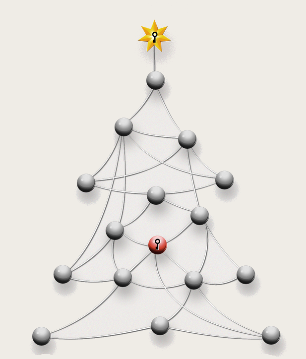
The task is about colouring the balls in blue, red or yellow in such a way that no two connected balls get the same colour. In mathematical terms, we are dealing with a graph colouring problem here – we have an undirected graph G = (V, E) with  nodes and  edges which needs to be coloured with the colours from the set C with colours. We already know the colour for two of the nodes. Hence, we are looking for an attribution of the colour to the nodes  such that the following criteria are met:

• Each node v is coloured with exactly one colour:

  

• No neighbour is coloured with the same colour

  

• is a binary variable:

To draw a connection between the Christmas tree and the resource allocation problem, we could think of the colours as the trains which need to run, the nodes as the resources and the edges as conflicts which prohibit the employment of a pair of resources on a given train (e.g. a driver not licensed for a given loco, a loco unable to operate on a given section of the network, etc.).

Such model formulations are frequently seen in the optimization of problems related to railways [1], [2], [3], [4]. They have primarily been used for train scheduling problems, e.g. helping dispatchers select the order in which trains should use platforms in a station. It is also popular as a modelling and optimization structure in other areas – it becomes increasingly useful as a method of optimizing the use of LTE transmission frequencies [5] [6].

After this small glimpse into my research, I wish you a blessed Christmas time this year, full of Lebkuchen (gingerbread) and Glühwein (mulled wine)!

 

References:

[1]  Lusby, Richard M., et al. “Railway Track Allocation: Models and Methods.” OR Spectrum, vol. 33, no. 4, 2009, pp. 843–883., doi:10.1007/s00291-009-0189-0.

[2] Cardillo, Dorotea De Luca, and Nicola Mione. “k L-List λ Colouring of Graphs.” European Journal of Operational Research, vol. 106, no. 1, 1998, pp. 160–164., doi:10.1016/s0377-2217(98)00299-9.

[3] Billionnet, Alain. “Using Integer Programming to Solve the Train-Platforming Problem.” Transportation Science, vol. 37, no. 2, 2003, pp. 213–222., doi:10.1287/trsc.37.2.213.15250.

[4] Cornelsen, Sabine, and Gabriele Di Stefano. “Track Assignment.” Journal of Discrete Algorithms, vol. 5, no. 2, 2007, pp. 250–261., doi:10.1016/j.jda.2006.05.001.

[5] Tsolkas, Dimitris, et al. “A Graph-Coloring Secondary Resource Allocation for D2D Communications in LTE Networks.” 2012 IEEE 17th International Workshop on Computer Aided Modeling and Design of Communication Links and Networks (CAMAD), 2012, doi:10.1109/camad.2012.6335378.

 

 

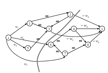
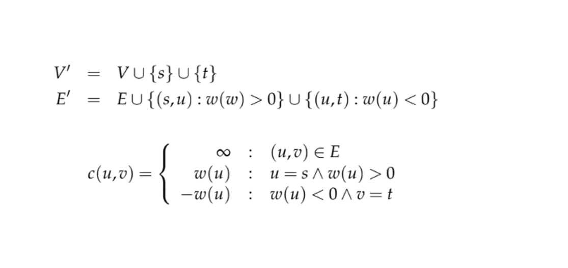Our beautiful new website is online