
by Umberto Morelli
In my first post on this blog, I gave a brief overview on the motivation and objectives of my PhD project. Briefly, we could summarize it as the estimation of the heat flux going from the steel in solidification to the mold during continuous casting. This heat flux is necessary in the process to cool down the liquid steel and trigger its solidification. With respect to the motivation, the reasons for doing that are basically to control the process and, eventually, know what is happening inside the mold, that would otherwise be just a black box.
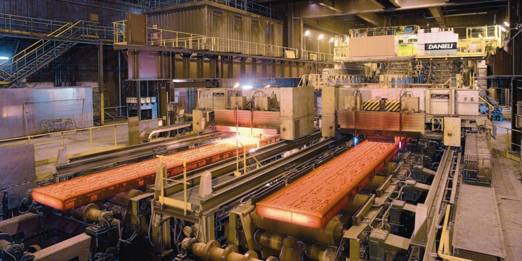
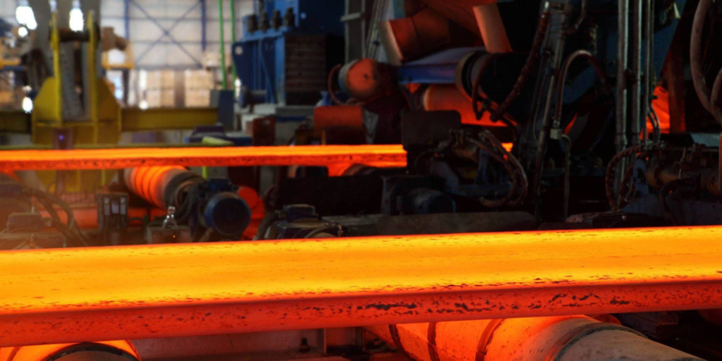
The first idea could be a hardware solution: we could equip the mold with some sensors on the “hot” face and measure the heat flux. Unfortunately, this is not possible. The hot face is not a place for sensors because of the critical temperature values and the abrasive effect of the sliding metal. However, casting molds are actually equipped with some kind of sensors.
In particular, they have thermocouples buried inside the mold plate a few centimeters inward with respect to the hot face. And these temperature measurements are gonna be the data of our problem.
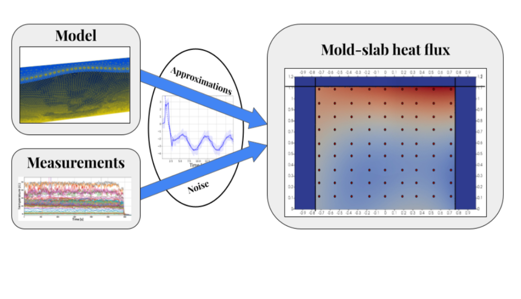
So the situation is the following: we have a set of temperature measurements and a mold thermal model (partial differential equation with some boundary conditions including the boundary heat flux). We want to combine these two ingredients to estimate the boundary heat flux. If we call the heat flux g, we have that the thermal model is a function F(g) that, given a heat flux g, provides the mold temperature, i.e.
g → F(g) → T
Where T is the mold temperature field. This is a classical “forward” problem in which we are given a boundary condition and we provide, solving some kind of model equations, the state of a system. However, our situation is somehow the opposite. We know the temperature at some points of our domain, Ť, and want to know the g. So we have something like
Ť → ? → g → F(g) → T
Then we are looking for an operator that allows us to go from Ť to g.
To do this we use an optimization approach. We decide that we are looking for a ĝ that minimize the difference between the measured temperature and the computed one, i.e.
Find ĝ such that (F(ĝ) – Ť) is minimized
There are several tools to solve such a minimization problem, however, all of them require several computations of the forward problem F(ĝ) that in our case is computationally expensive and requires several minutes. However, since the objective is to control the casting process, we want to have the solution in “real-time” i.e. in very little time allowing us to detect problems and reach in time (approximately one second).
To find the solution of this problem in real-time, we exploit the affinity of the direct problem. In fact, we have that if we assume that g can be somehow parameterized like
g = a1φ1+ a2φ2+…+aNφN
for some basis functions φ1, φ2,…,φN. Then, the solution of the direct problem is given by
T = a1F(φ1)+a2F(φ2)+…+aNF(φN)+C
where C is something that we must add to obtain the correct solution.
Skipping all the mathematical details, this affinity allows us to find the minimizer of (F(ĝ) – Ť) in a very simple way, i.e. by solving a linear system having the dimension of the parameterization of the heat flux g. Moreover, to assemble the linear system, we only have to compute the direct problem for all the parameterization basis F(φ1), F(φ2),..,F(φN).
These last computations are expensive but can be done once and for all at the beginning during an offline phase. While, in a very fast online phase, we only solve the little linear system which is a fast and inexpensive computation.
Also in this case then, the offline-online decomposition, which is the core of model order reduction, allows us to achieve real-time performances in the solution of a problem that in the classical setting is very time consuming. I invite the interested reader to have a look at our recent publication on the subject at the link.